On this page

In the previous post, we introduced the core idea of Hidden Decoding: without increasing the parameters of the Transformer backbone, we replicate the Vocab Embedding $n$ times to expand the sequence length by a factor of $n$, giving each token $n$ times the effective computation in a single forward pass — and we validated the loss reductions and benchmark gains at 6B, 8B, and 80B scales. This post is the sequel: we push Hidden Decoding to frontier scale (100B+ MoE), training WeLM-HD4-80B and WeLM-HD4-617B ($n=4$), which improve their matched autoregressive baselines across the board in fully controlled comparisons, and we present the key engineering designs that make the method actually trainable and servable at very large scale. The full paper for this work is available at Tencent/Sequential-Hidden-Decoding.

Two headline conclusions:

1. Frontier-scale fixed-backbone scaling. To our knowledge, this is the first demonstration of sequence-length scaling at the 100B+ MoE scale through continued pretraining (CPT) — a regime not reached by prior depth-recurrent (looped) or length-scaling approaches.
2. Stream-Factorized Attention makes the expansion trainable at scale. Most layers attend only within a stream and only a few layers mix across streams, reducing the added attention cost from $O(n^2)$ to roughly linear, so Hidden Decoding can be trained and served at the 100B+ MoE scale at an acceptable cost.

Figure 1: Left: Hidden Decoding expands each token into multiple streams along the sequence (shown with an expansion factor of 2), processed in a single forward pass, with the loss applied only at each token’s final stream ($E_2/h_2$) while the earlier streams ($E_1/h_1$) act as latent intermediate computation with no loss. Right: improvement $\Delta$ (in points) of WeLM-HD4-80B and WeLM-HD4-617B over their matched autoregressive baselines (WeLM-80B / WeLM-617B) under the same early SFT-only post-training.

Frontier-Scale MoE Results

To test whether Hidden Decoding strengthens the largest models we deploy, we compare two forms of each WeLM MoE checkpoint that share everything except Hidden Decoding: WeLM-80B (3B activated) vs. WeLM-HD4-80B, and WeLM-617B (23B activated) vs. WeLM-HD4-617B. Both forms are then adapted with the same early SFT-only post-training recipe (short SFT, no RL), so this is a single-variable ablation of the Hidden Decoding method.

Benchmark	80B MoE		617B MoE		External
	WeLM-80B	WeLM-HD4-80B	WeLM-617B	WeLM-HD4-617B	Kimi K2.6 (1T-A32B)
GPQA Diamond	87.6	88.8	89.1	91.2	90.4
HLE†	27.4	28.4	33.6	35.4	36.9
MMMLU	84.4	85.6	86.4	87.5	88.0
FrontierMath*	45.8	49.0	49.0	51.0	53.2
PHYBench	69.8	73.8	75.3	76.3	74.0
MathArena Apex	16.4	20.1	24.2	24.7	23.8
HMMT‡	93.3	94.1	96.0	96.2	96.0
IMO-AnswerBench	85.0	85.3	87.5	88.5	91.5
SciCode	45.8	50.0	51.4	52.1	50.7

Table 1: Early SFT-only results. Each WeLM-HD4 model (highlighted) is compared with its matched autoregressive counterpart under the same short SFT recipe (no RL); HD4 denotes Hidden Decoding with $n=4$ and unchanged active Transformer parameters per token (3B for 80B, 23B for 617B). Kimi K2.6 is listed as a mainstream frontier-model reference for absolute score scale. All numbers in this table are from our own evaluation. *FrontierMath uses the public Tiers 1–4 sample problems (epoch.ai/frontiermath/tiers-1-4/benchmark-problems). †HLE uses a no-tools, text-only setting. ‡HMMT is the weighted average over the Feb. 2025, Nov. 2025, and Feb. 2026 sets.

Hidden Decoding improves all nine shared benchmarks at both scales. The largest gains appear on hard math and science tasks: WeLM-HD4-80B improves SciCode by +4.2, PHYBench by +4.0, and FrontierMath by +3.2; WeLM-HD4-617B improves GPQA Diamond by +2.1 and HLE by +1.8. We also report our own evaluation of Kimi K2.6 (1T total, 32B activated) under the same testing setting as a mainstream frontier-model reference for absolute scale (Moonshot AI 2026): WeLM-HD4-617B is higher on GPQA Diamond, PHYBench, MathArena Apex, HMMT, and SciCode. These results show that Hidden Decoding can scale to frontier-size MoE models and improve them without adding backbone parameters — the regime where looped models are hard to apply.

We place WeLM-HD4-617B-Base’s base model in the base-model reference of external models. We primarily focus on the autoregressive-vs-HD comparison under the same backbone, data, and training configuration.

Benchmark	WeLM-617B-Base	WeLM-HD4-617B-Base	DS-V3.2 671B-A37B	K2 1T-A32B	Qwen3.5 397B-A17B
MMLU	89.80	90.40	88.11	87.38	88.61
MMLU-Pro	71.00	72.80	62.82	67.64	76.01
MMLU-Redux	89.81	90.94	87.29	86.65	89.09
SuperGPQA	55.70	57.60	43.46	44.86	57.96
C-Eval	92.20	92.80	90.48	91.82	91.82
BBH	92.41	93.07	86.03	89.11	90.98
KoRBench	52.08	54.88	54.00	53.84	54.08
CRUX-Input	86.00	91.75	63.25	70.50	71.13
CRUX-Output	89.38	91.13	73.88	77.13	82.38

Table 2: Base-model reference. The WeLM columns use our base-model protocol before instruction tuning or RL; the matched WeLM-617B-Base vs. WeLM-HD4-617B-Base pair gives the controlled autoregressive-vs-HD comparison, while the external numbers are copied from the Qwen3.5 report’s base-model table for absolute-score context (Qwen Team 2026).

Moreover, the gains appear before post-training: the full-suite average rises by +0.99 on 80B and +1.03 on 617B, with the larger gains on harder reasoning and knowledge tasks such as SuperGPQA and MMLU-Pro, and they persist after the same lightweight post-training.

Method Recap and New Designs

Multi-Stream Expansion and Training Objective

Given an input sequence $X=(x_1,\dots,x_L)$ and $n$ embedding tables $E_1,\dots,E_n$, we place the stream-$k$ representation of token $x_i$ at physical position $t=(i-1)n+k$, forming an expanded sequence of length $nL$: $$ S_t = E_k(x_i), \quad 1 \le i \le L,\ 1 \le k \le n. $$ The expanded sequence is fed to the same Transformer under standard causal attention with contiguous RoPE positions. Only the final stream $E_n(x_i)$ of each token is supervised: the next token $x_{i+1}$ is predicted from its hidden state through the shared LM head, while the first $n-1$ streams receive no direct loss and act as latent intermediate computation that progressively refines the representation. For why final-stream supervision beats all-token loss / sum, and for the Cyclic Replication Initialization used for progressive expansion $1\to2\to4\to8$, see the previous post.

Stream-Factorized Attention

Keeping full cross-stream attention at all layers makes attention cost grow as $O(n^2)$, which is infeasible to train for large models with long sequences. We therefore propose Stream-Factorized Attention: most layers attend only within a stream, and only a few layers mix across streams.

For a position $t$ in the expanded sequence, define its token and stream indices: $$ i(t)=\lceil t/n \rceil, \quad s(t)=(t-1)\bmod n + 1. $$ An intra-stream layer restricts attention to earlier positions of the same stream, costing $O(nL^2)$; a cross-stream layer also attends across streams, following the base model’s usual attention pattern (sliding-window, or full when the base model uses full attention).

Figure 2: The three attention masks in Stream-Factorized Attention. (a) A full cross-stream layer uses the standard causal (lower-triangular) mask; (b) a local cross-stream layer uses a causal sliding-window mask; (c) an intra-stream layer is causal within each stream, so streams are invisible to one another. Most layers are (c), with cross-stream mixing (a or b) enabled at only a few layers.

By design, the vast majority of layers are intra-stream, and cross-stream attention is enabled at only a small subset of layers — and we add no new attention layers: we enable cross-stream attention on all local-attention layers and a small subset of full-attention layers. Because dense attention over the full $nL$ sequence is avoided at most layers, the added attention cost drops from quadratic to roughly linear in $n$ — this is what makes Hidden Decoding trainable at the 100B+ MoE scale. This layout, where most layers keep the single-stream causal path and only a few introduce cross-stream perturbations, also keeps CPT closer to the starting autoregressive checkpoint, giving a smoother startup.

Persistent KV and the KV-mirror Saving

Persistent intermediate-stream KV. Hidden Decoding retains a separate KV cache per stream, so later positions can use the computation produced by earlier intermediate streams. We run this ablation in the Ablations and Probes section. Moreover, by introducing stream parallelism, we shard the intra-stream KV across different ranks, reducing the storage and memory-access pressure of the KV.

KV-mirror training speedup. Our WeLM backbones use a KV-mirror design (WeChat AI 2026): each later layer computes its keys and values from an earlier layer’s hidden states (layers paired in a U-shape, with the last third mirroring the first third). Because a mirrored layer’s K/V depend only on the early layers’ hidden states, and only the final stream is supervised (intermediate streams matter only through the K/V they add), in the mirrored layers this context is already fixed and the intermediate streams need not be processed. We therefore run only the final stream through the mirrored layers while early layers still process all $n$ streams. In an 80B, 32k training setting this reduces per-batch time from 15s to 12s (a 20% reduction, 1.25×). This saving is specific to WeLM, on top of the near-linear cost that Stream-Factorized Attention already provides.

Computational Cost

Near-Linear Training Cost

Expanding each token into $n$ streams turns a length-$L$ sequence into $nL$: non-attention computation scales roughly with the number of positions, while dense attention would blow up as $O(n^2)$. Stream-Factorized Attention avoids this by keeping most full-attention layers intra-stream, so the attention cost stays close to linear in $n$.

Figure 3: Per-batch training time of HD ($n=4$) relative to the unexpanded baseline: 5.1× on 80B (256k→1M) and 4.4× on 617B (32k→128k), close to the linear reference ($n=4\times$) and far below dense attention ($n^2=16\times$).

Measurements confirm the analysis: a $4\times$ effective sequence costs 5.1× on 80B and 4.4× on 617B, close to the $4\times$ linear reference and far below the $16\times$ dense-attention cost. This near-linear cost is what makes WeLM-HD4-617B trainable.

More importantly, HD4 is not trained from scratch but continues training from an existing autoregressive base checkpoint: it only trains after the HD start point and does not rerun the full 8k pretraining stage. As a result, counting only the tokens after the HD start point, HD4’s total training cost is far below training a full autoregressive base from scratch — 1.07T vs. 20.39T on 80B, and 0.90T vs. 17.06T on 617B.

Scale	Run	HD start tokens	8k pretrain	32k continuation	256k continuation	Total
80B	WeLM-80B-Base	–	17.81T	2.01T	0.57T	20.39T
80B	WeLM-HD4-80B-Base	19.32T	0	0.50T	0.57T	1.07T
617B	WeLM-617B-Base	–	14.25T	2.20T	0.61T	17.06T
617B	WeLM-HD4-617B-Base	15.86T	0	0.59T	0.30T	0.90T

Table 5: Training-token budgets for autoregressive base paths and HD4 continuation windows. Autoregressive rows count the full base-model path; HD4 rows count only the training after the HD start point.

Inference Throughput

A key advantage over looped models is that Hidden Decoding’s extra computation runs in parallel: a looped model repeats the backbone step by step and each step waits for the previous one, so the cost cannot be hidden; Hidden Decoding spreads its computation across the $n$ streams processed together in a single pass. At large batch sizes decoding is compute-bound and the extra computation lowers throughput (as it must for any method that adds computation); but at small batch sizes decoding is memory-bandwidth-bound with idle compute, and the parallel streams run on that idle compute.

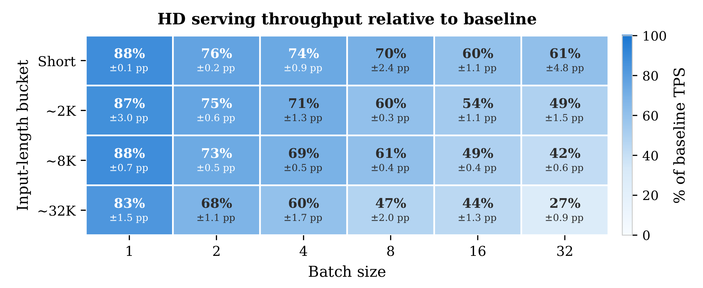Figure 4: Serving throughput matrix for WeLM-HD4-80B. Each cell is Hidden Decoding’s decoding-only completion throughput as a percentage of the matched WeLM-80B baseline (stream expansion disabled), averaged over five runs under the same input-length bucket and batch size (small text: sample std. in pp). Both run on the same 8×H20 GPUs; prefill is excluded.

Ablations and Probes

Hidden Decoding relies on an unusual choice: only the final stream is trained to predict the next token, while the earlier streams receive no direct loss. The main results show this improves accuracy, but the accuracy gain alone does not reveal the role of the intermediate streams — a gain could come from simpler effects such as a longer sequence, more prediction targets, or explicit aggregation of stream outputs. We use ablations and probes to separate these possibilities.

Attention-Composition Ablation

Stream-Factorized Attention saves cost by limiting expensive full cross-stream mixing, so we test how much full mixing is required for accuracy. On the 21B MoE (27 layers), three Hidden Decoding variants differ only in how many layers use full cross-stream mixing (all 27, 4, or 1), with the remaining layers split between local and intra-stream mixing; the reference is a no-expansion autoregressive baseline.

Benchmark	Baseline	Hidden Decoding
		SF (1 full)	SF (4 full)	all-full (27)
MMLU	74.1	75.7	76.4	76.3
MMLU-Pro	47.5	50.4	49.8	50.7
CMMLU	77.9	79.2	79.8	79.6
C-Eval	78.6	78.9	79.2	79.7
ARC-C	89.5	89.8	90.7	90.9
SuperGPQA	34.1	35.4	35.7	36.0
BBH	67.0	71.2	72.0	72.8
GSM8K	83.4	86.2	86.7	86.2
MATH	45.2	49.6	49.3	50.3
SimpleQA	3.7	4.0	3.6	4.1
AA-OmniScience	12.7	12.4	14.2	14.1
HumanEval+	37.4	37.6	39.2	40.5
MBPP+	55.2	56.1	57.8	59.1
Overall (13 tasks)	54.33	55.88	56.49	56.95

Table 3: Attention-composition ablation (21B MoE). All Hidden Decoding variants improve substantially over the no-expansion autoregressive baseline, and the Stream-Factorized (SF) variants with only 1 or 4 full-attention layers nearly match the all-full configuration. Header parentheses give the number of full-attention layers (out of 27); the overall average is over the 13 benchmarks listed. Best value in each row in bold.

Every Hidden Decoding model beats the autoregressive baseline by a wide margin (overall gains +1.55 to +2.62). The all-full model is best, but the cheaper 4-full and 1-full variants recover most of the gain (+2.16 and +1.55). A few full layers are enough: the remaining cross-stream mixing can be local or skipped, which keeps Stream-Factorized Attention cheap while preserving most of the accuracy gain.

KV Retention Ablation

For KV retention, we run a qualitative control on the 21B MoE at $n=2$: replacing per-stream KV with a shared KV (keeping the final-stream objective and separate stream trajectories, but using one shared KV in intra-stream layers). Shared KV lowers the average in both layouts (SF-1full: 69.00 → 68.59; SF-4full: 69.46 → 69.06), indicating that keeping separate KV states per stream helps.

Full layers	KV type	Few-shot accuracy						Avg
		ARC	EEGPQA	MMLU	MMLU-Pro	QA-MMLU	SuperGPQA
1	Per-stream	91.50	54.17	74.62	48.83	80.90	35.36	69.00
	Shared	91.01	53.19	74.24	46.60	81.07	34.63	68.59
4	Per-stream	92.32	54.95	75.24	47.82	82.11	35.50	69.46
	Shared	91.28	53.32	74.41	47.90	81.15	35.35	69.06

Table 4: Small KV-retention ablation (21B MoE, HD $n=2$). A qualitative check of whether stream-specific KV matters. Accuracy columns are few-shot accuracy in percent (higher is better); Avg is over all nine few-shot tasks. Per-stream KV wins on average in both layouts.

Stream and LM-head Probes

To connect these accuracy effects to internal computation, we probe the trained Qwen3-8B-Base + Hidden Decoding model at $n=8$ (E7 the final prediction stream, E0–E6 intermediate), and reach two consistent conclusions.

First, the intermediate streams form distinct internal states that the final stream reads. Same-token streams separate markedly in the Transformer’s middle layers and partially move closer near the output (mean cosine 0.987→0.637→0.783), staying above the different-token baseline throughout; meanwhile the final stream E7 assigns substantial attention to other streams (especially E0, peaking at 0.52), forming a read path from the intermediate streams to the prediction stream (Figure 5).

Figure 5: Probes on Qwen3-8B-Base + Hidden Decoding ($n=8$). (a) Cosine similarity of same-token streams’ hidden states across Transformer layers (dashed: different-token baseline). (b) Attention mass the final stream E7 assigns to each stream.

Second, in vocabulary space the intermediate streams keep a broader candidate distribution than the final stream. Applying the shared LM head to each stream, intermediate streams’ top-1 token often differs from E7 (largest difference rate ~63%), and their probe entropy is generally higher than the final stream’s, indicating broader token-level uncertainty before the prediction consolidates (Figure 6).

Figure 6: Next-token distributions from applying the shared LM head to each stream’s hidden state. (a) Fraction of intermediate probes whose top-1 differs from E7. (b) Mean probe entropy per stream ($n=2,4,8$).

Taken together, the ablations and probes point to the same interpretation: the training-objective ablation shows final-stream supervision beats supervising every stream or summing outputs; the KV and attention analyses show per-stream KV is useful, streams separate inside the Transformer, and the final stream reads the others; the LM-head probes give a vocabulary-space view — intermediate streams keep a broader candidate set before the final stream consolidates it into a prediction. This is the sense in which Hidden Decoding uses the earlier streams as latent computation states.

Conclusion and Future Work

This post pushes Hidden Decoding from method validation to frontier scale. By expanding along the sequence dimension with Stream-Factorized Attention, we train WeLM-HD4-80B and WeLM-HD4-617B at $n=4$, improving their matched autoregressive baselines across the board under the same early SFT-only post-training; the training-cost measurements explain why this scale is practical. Together, these results establish sequence-length expansion as a practical fixed-backbone scaling path for frontier-scale LLMs.

Looking ahead, we will keep pushing Hidden Decoding on top of stronger baselines. After post-training on higher-quality and larger-scale data, the 80B and 617B autoregressive MoE bases already show markedly higher benchmark scores and a more stable user experience (Table 6); next, we will further validate Hidden Decoding’s gains on these stronger baselines and fully combine it with RL to keep extending the models’ capability frontier.

Benchmark	Kimi K2.6	WeLM-80B	WeLM-617B
AA-LCR	76.00	72.60	74.80
AA-Omniscience	36.50	29.58	38.00
SciCode	50.69 (52.2)	47.29	52.22
ARC-AGI-2	24.72	8.33	30.42
Chinese Writing§	92.35	87.92	91.66
FrontierMath*	53.21	47.83	56.68
GPQA Diamond	90.40 (90.5)	89.80	91.21
HLE†	36.90 (36.4)	31.90	38.40
HMMT‡	95.97	94.35	95.70
IFBench	76.67	71.93	75.87
IMO-AnswerBench	91.50 (86.0)	88.00	94.00
LiveCodeBench v6	86.86 (89.6)	84.76	88.57
MathArena Apex	23.78	38.98	60.24
MMMLU	87.96	84.61	88.11
Multilingual-Open§	74.60	69.26	73.59
PHYBench	74.00	76.12	75.00
Terminal-Bench 2.1	65.4	61.05	74.2

Table 6: Benchmark results of the new autoregressive MoE bases post-trained on higher-quality, larger-scale data; Kimi K2.6 is included as a mainstream frontier-model reference. All scores are in percent. The Kimi K2.6 column is our own evaluation under the same harness as WeLM, with the officially reported score in parentheses where available.

• *FrontierMath uses the public Tiers 1–4 sample problems.
• †HLE uses a no-tools, text-only setting.
• ‡HMMT is the weighted average over the Feb. 2025, Nov. 2025, and Feb. 2026 sets.
• §Chinese Writing and Multilingual-Open are internal datasets.
• Terminal-Bench 2.1: evaluated using the Terminus-2 framework with the provided JSON parser; decoding used temperature=1.0, top_p=0.95, and a 256K context window, averaged over two independent runs.

References

Moonshot AI. 2026. Kimi K2.6. https://huggingface.co/moonshotai/Kimi-K2.6.
Qwen Team. 2026. Qwen3.5. https://qwen.ai/blog?id=qwen3.5.
WeChat AI. 2026. Building Effective Sparse MoE Models with Moderate Resources. https://welm.weixin.qq.com/posts/building-effective-sparse-moe-models-with-moderate-resources/.